Predictionphase
Prediction Phase
Contents
Prepare loading functions
The computation of URFs concludes the construction phase of NPSAT. Now we can use the URFs to make prediction for any given loading function.
In this illustration we will assume the following:
- The stream recharge is clean e.g. zero concentration
- The loading is spatialy unifom but varies over the years
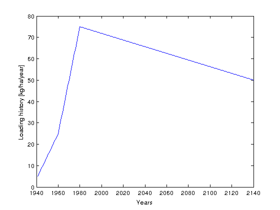
- From 1941 - 1980 a slight increase of loading from 5 to 25 kg/ha/year
- From 1980 - 2000 an large increate from 25 to 75 kg/ha/year
- A steady slight decrease from 2000 to the end of simulation time (2140)
years = [1941:2140];
LF = zeros(1,200);
LF(1:20) = linspace(5,25,20);
LF(20:40) = linspace(25,75,21);
LF(40:end) = linspace(75,50,161);
plot(years, LF)
ylabel('Loading history [kg/ha/year]')
xlabel('Years')

In case you continue from the previous tutorials you can skip this step. Here we only load the data of the previous steps.
the particle tracking data
load NPSAT_Streamline_Data
and the unit response function data.
load NPSAT_URFs
First we need to convert the loading history from Mass to concentration by dividing the the loading with hte groundwater recharge. We will loop through the streamlines and identify the recharge rates that correspond to the last point of the streamline. Note that the last point is the exit point of the streamline near the water table, while the first point is the near the well. We will also compute the velocity of the streamline near the well.
For the domestic wells We allocate space to hold the velocities
Vel_dm = zeros(size(XYZdm,1),1);
and hold the recharge
Rch_dm = zeros(size(XYZdm,1),1);
for i = 1 : size(XYZdm,1)
    endpnt = XYZdm{i,1}(end,:);
    %check if it is close to stream
    if endpnt(1)>=4970 && endpnt(1)<=5030;
        Rch_dm(i,1) = 0;
    else
        if endpnt(2) <= 10000
            Rch_dm(i,1) = 1e-4;
        elseif endpnt(2) <= 20000
            Rch_dm(i,1) = 2e-4;
        elseif endpnt(2) <= 30000
            Rch_dm(i,1) = 3e-4;
        else
            Rch_dm(i,1) = 4e-4;
        end
    end
    Vel_dm(i,1) = sqrt(sum(Vdm{i,1}(1,:).^2));
end
Similarly for the irrigation wells
Vel_ir = zeros(size(XYZir,1),1);
Rch_ir = zeros(size(XYZir,1),1);
for i = 1 : size(XYZir,1)
    endpnt = XYZir{i,1}(end,:);
    %check if it is close to stream
    if endpnt(1)>=4970 && endpnt(1)<=5030;
        Rch_ir(i,1) = 0;
    else
        if endpnt(2) <= 10000
            Rch_ir(i,1) = 1e-4;
        elseif endpnt(2) <= 20000
            Rch_ir(i,1) = 2e-4;
        elseif endpnt(2) <= 30000
            Rch_ir(i,1) = 3e-4;
        else
            Rch_ir(i,1) = 4e-4;
        end
    end
    Vel_ir(i,1) = sqrt(sum(Vir{i,1}(1,:).^2));
end
Next we will create the loading functions. ie we will convert the loading function form mass to concentration
First we convert the recharge from m/day to m/year
Rch_dm = Rch_dm * 365;
Rch_ir = Rch_ir * 365;
Then we convert it to m^3/ha/year
Rch_dm = Rch_dm*10000;
Rch_ir = Rch_ir*10000;
and then divide the Mass with the recharge to get concentration
LF_dm = bsxfun(@rdivide, LF,Rch_dm);
LF_ir = bsxfun(@rdivide, LF,Rch_ir);
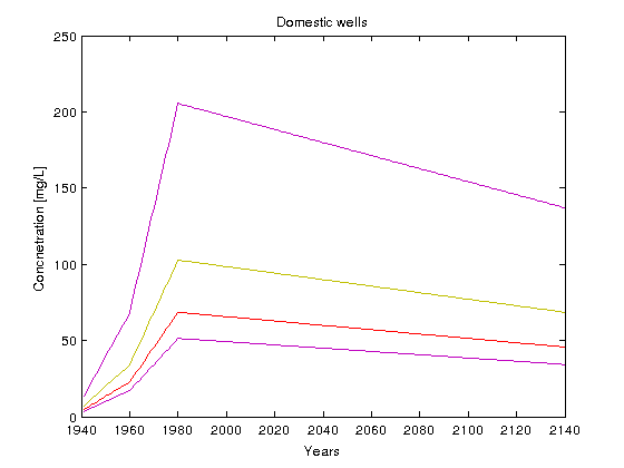
Therefore the real loading functions are actually grouped into 4 categories as shown below
plot(years,1000*LF_dm');ylabel('Concnetration [mg/L]');
xlabel('Years'); title('Domestic wells')

Convolution
Once the loading functions are in the approprieate format we convolute them with the URFs.
For each well we first identify the id of streamlines that correspond to, We perform the convolution operator and compute the average well breakthrough curve based on the flow contribution of each streamline. The flow contribution is taken analogous the the velocity of the streamline at the well. Note that the particles are uniformly distributed around the well screen length therefore the flow contribution of each streamline is equal to the velocity (The area is the same for all the streamlines)
The main convolution loop for the domestic wells:
for i = 1: max(well_id_dm)
    id = find(well_id_dm == i);
    load_func = LF_dm(id,:);
    urfs = URFdm(id,:);
    temp_BTC = ConvoluteURF(urfs,load_func,'cpp');
    BTCdm(i,:) = sum(bsxfun(@times, temp_BTC, Vel_dm(id,1)),1)./sum(Vel_dm(id,1));
end
and we repeat for the irrigation wells
for i = 1: max(well_id_ir)
    id = find(well_id_ir == i);
    load_func = LF_ir(id,:);
    urfs = URFir(id,:);
    temp_BTC = ConvoluteURF(urfs,load_func,'cpp');
    BTCir(i,:) = sum(bsxfun(@times, temp_BTC, Vel_ir(id,1)),1)./sum(Vel_ir(id,1));
end
Next we will create 4 groups of wells for the domestic and irrigation wells. First we group the x-y coordinates into domestic and irrigation
cntdm = 1;
cntir = 1;
for i = 1:size(wells,1)
    if strcmp(wells(i,1).desc,'dom')
        xy_dm(cntdm,:) = [wells(i,1).X wells(i,1).Y];
        cntdm = cntdm +1;
    elseif strcmp(wells(i,1).desc,'irr')
        xy_ir(cntir,:) = [wells(i,1).X wells(i,1).Y];
        cntir = cntir +1;
    end
end
and then we will group them according to the recharge zone and plot
well_zone{1,1} = find(xy_dm(:,2) <= 10000);
well_zone{1,2} = find(xy_ir(:,2) <= 10000);
well_zone{2,1} = find(xy_dm(:,2) > 10000 & xy_dm(:,2) <= 20000);
well_zone{2,2} = find(xy_ir(:,2) > 10000 & xy_ir(:,2) <= 20000);
well_zone{3,1} = find(xy_dm(:,2) > 20000 & xy_dm(:,2) <= 30000);
well_zone{3,2} = find(xy_ir(:,2) > 20000 & xy_ir(:,2) <= 30000);
well_zone{4,1} = find(xy_dm(:,2) > 30000);
well_zone{4,2} = find(xy_ir(:,2) > 30000);
subplot(2,1,1);hold on
zone1Lines = plot(years,1000*BTCdm(well_zone{1,1},:),'r');
zone2Lines = plot(years,1000*BTCdm(well_zone{2,1},:),'b');
zone3Lines = plot(years,1000*BTCdm(well_zone{3,1},:),'g');
zone4Lines = plot(years,1000*BTCdm(well_zone{4,1},:),'c');
zone1group = hggroup;
zone2group = hggroup;
zone3group = hggroup;
zone4group = hggroup;
set(zone1Lines,'Parent',zone1group)
set(zone2Lines,'Parent',zone2group)
set(zone3Lines,'Parent',zone3group)
set(zone4Lines,'Parent',zone4group)
set(get(get(zone1group,'Annotation'),'LegendInformation'),'IconDisplayStyle','on');
set(get(get(zone2group,'Annotation'),'LegendInformation'),'IconDisplayStyle','on');
set(get(get(zone3group,'Annotation'),'LegendInformation'),'IconDisplayStyle','on');
set(get(get(zone4group,'Annotation'),'LegendInformation'),'IconDisplayStyle','on');
axis([1940 2140 0 200])
ylabel('Concentration [mg/L]')
title('BTCs for domestic wells')
grid on
legend('Zone 1e-4','Zone 2e-4','Zone 3e-4','Zone 4e-4','Location','EastOutside')

subplot(2,1,2);hold on
zone1Lines = plot(years,1000*BTCdm(well_zone{1,2},:),'r');
zone2Lines = plot(years,1000*BTCdm(well_zone{2,2},:),'b');
zone3Lines = plot(years,1000*BTCdm(well_zone{3,2},:),'g');
zone4Lines = plot(years,1000*BTCdm(well_zone{4,2},:),'c');
zone1group = hggroup;
zone2group = hggroup;
zone3group = hggroup;
zone4group = hggroup;
set(zone1Lines,'Parent',zone1group)
set(zone2Lines,'Parent',zone2group)
set(zone3Lines,'Parent',zone3group)
set(zone4Lines,'Parent',zone4group)
set(get(get(zone1group,'Annotation'),'LegendInformation'),'IconDisplayStyle','on');
set(get(get(zone2group,'Annotation'),'LegendInformation'),'IconDisplayStyle','on');
set(get(get(zone3group,'Annotation'),'LegendInformation'),'IconDisplayStyle','on');
set(get(get(zone4group,'Annotation'),'LegendInformation'),'IconDisplayStyle','on');
axis([1940 2140 0 200])
xlabel('Years')
ylabel('Concentration [mg/L]')
title('BTCs for irrigation wells')
grid on
legend('Zone 1e-4','Zone 2e-4','Zone 3e-4','Zone 4e-4','Location','EastOutside')
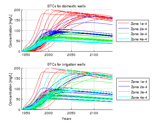
We can observe that the recharge zone influence significantly the domestic wells because the source area of shallow wells with short screen lengths is very small, therefore it is quite likely that the source area is with the recharge zone that the well belongs to. On the other hand the source area of deep wells can be very large and it may span more than 2 different recharge zones. Therefore the BTCs are quite similar for all the wells independently of the recharge zone.

